A complete walkthrough of the SisMOM desktop application — from installation to running your first simulation. Video tutorials are coming soon; this written guide is the fastest way to get started today.
Overview
STFM simulates the trajectory and behavior of oil slicks spilled at sea. Once petroleum is released at the sea surface, it is transported by currents, winds, and waves, while simultaneously undergoing physicochemical processes that change its properties: evaporation of the lighter fractions, horizontal spreading due to gravity, seawater entering the oil (emulsification), and dispersion of droplets into the water column. STFM represents the spill as a set of particles that move individually in response to these environmental forcings, making it possible to estimate which coastal areas will be affected and when.
The typical workflow follows this order:
Installation → Open the app → New project → Grid → Downloader → Converter → Simulation
The grid must be created before downloading data, because the Converter needs it to clip the data to the area of interest. Data must be downloaded before conversion, which in turn must be completed before running the simulation.
1. Installation
Locate the STFM.msi file and double-click to open the installer.
Follow the installation wizard and click Next until it finishes.
When it's done, the STFM shortcut appears on the desktop.
Figure 1: STFM shortcut on the desktop
2. Opening STFM
Double-click the STFM icon on the desktop.
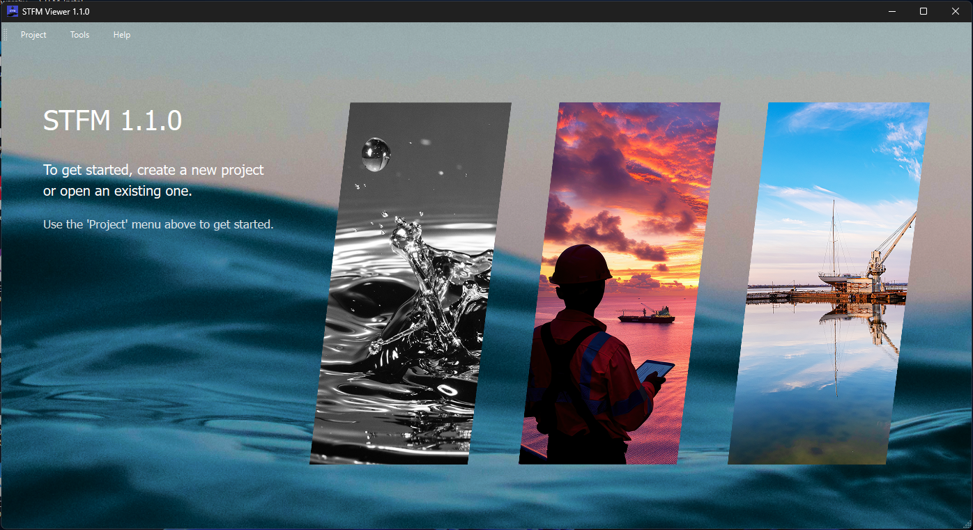
The start screen is displayed with the message "To get started, create a new project or open an existing one."
At this point, only the Project menu is available in the top bar. The Tools and Help menus appear only after a project has been opened.
Figure 2: STFM start screen
3. Creating or opening a project
New project
In the top bar, click Project.
In the menu that opens, click New Project.
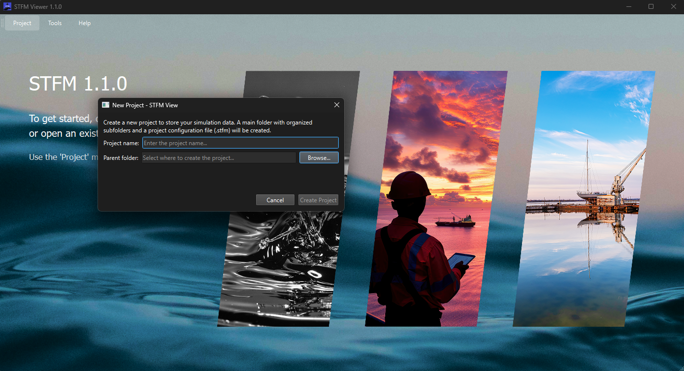
In the window that appears, fill in:
Project Name: type the project name
Folder: click Browse and choose the folder where the project will be saved
Click Create Project.
Figure 3: New project creation window
STFM automatically creates the following folder structure inside the chosen folder:
Project Name/
├── RAW_DATA/      ← raw files downloaded by the Downloader
├── CURRENTS/      ← converted currents, ready for the simulation
├── WINDS/         ← converted winds, ready for the simulation
├── WAVES/         ← converted waves, ready for the simulation
├── TEMPERATURE/   ← temperature and salinity (3D simulations)
├── OUTPUTS/       ← results generated after the simulation
├── GRIDS/         ← computational grid files
├── CONFIG/        ← saved simulation parameters
└── ANALYSIS/      ← coastal distribution analyses
Opening an existing project
In the top bar, click Project.
Click Open Project.
Browse to the project folder and select the .stfm file.
Click Open.
4. Main interface
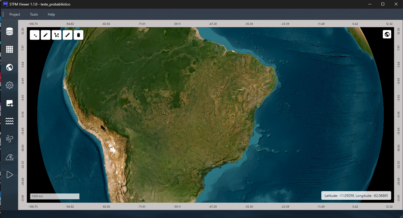
Once a project is created or opened, the main interface is displayed.
Figure 4: Main interface with map and sidebar
The interface has three elements:
Top bar (menus)
Project: New, Open, Save, Close project, Exit
Tools: Downloader, Converter
Help: Coefficients, Help, About
Interactive map
Occupies the central area of the screen. It displays the region of interest with all active layers. In the upper-left corner of the map there are buttons to interact directly with it:
First button: draw polygon on the map (used to delimit the spill area or reclassify land use)
Second button: add point on the map (used to mark the spill point)
Third button: create grid from the map (an alternative to filling in coordinates manually in the Grids panel)
Fourth button: erase what was drawn
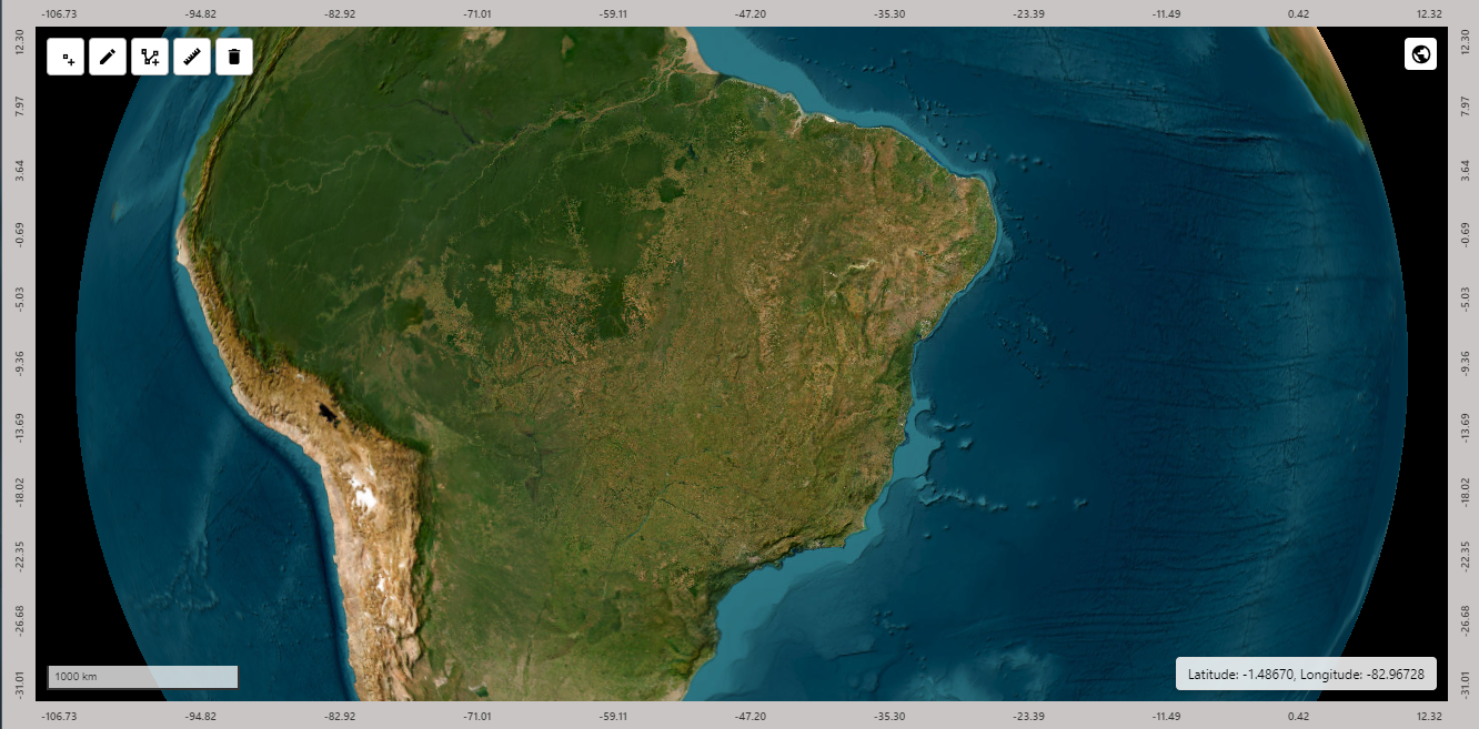
Button in the upper-right corner: toggle between Globe and Mercator projection
Figure 5: Interactive map buttons
Left sidebar (panels)
A column of icons on the left side of the screen. Click any icon to open the corresponding panel. Click it again to close it.
Panel
Function
Layers
Controls visibility, opacity, and playback of animated sequences
Grids
Creates the computational grid that defines the simulation area and resolution
Land Use
Land cover classification: identifies water and land cells
Settings
Simulation parameters, oil properties, and spill placement
Raster
Overlays georeferenced images on the map for visual reference
Currents
Loads and displays ocean current data
Winds
Loads and displays atmospheric wind data
Waves
Loads and displays wave data
Run
Checks project files and runs the simulation
5. Panel: Layers
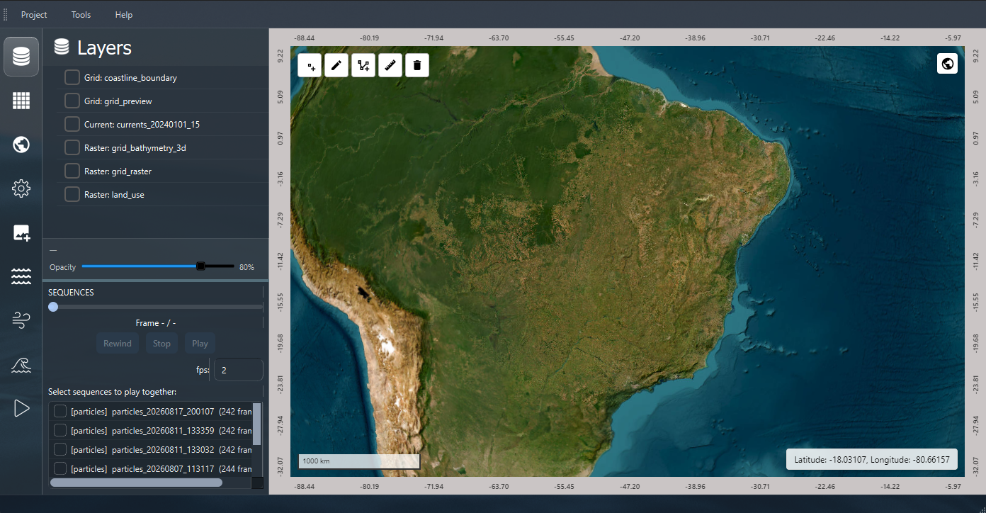
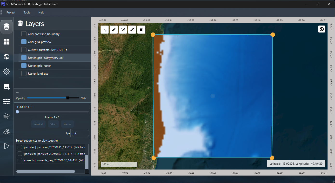
The Layers panel controls what appears on the map and manages playback of the animated sequences generated in the Currents, Winds, and Waves panels.
Click the Layers icon in the sidebar to open the panel.
Figure 6: Layers panel open
To show or hide a layer:
Check or uncheck the checkbox next to the layer name.
To adjust a layer's opacity:
Click the desired layer to select it.
Move the opacity slider (0–100%) to the desired value.
To reorder layers:
Click and drag the layer name up or down the list.
To play animated sequences:
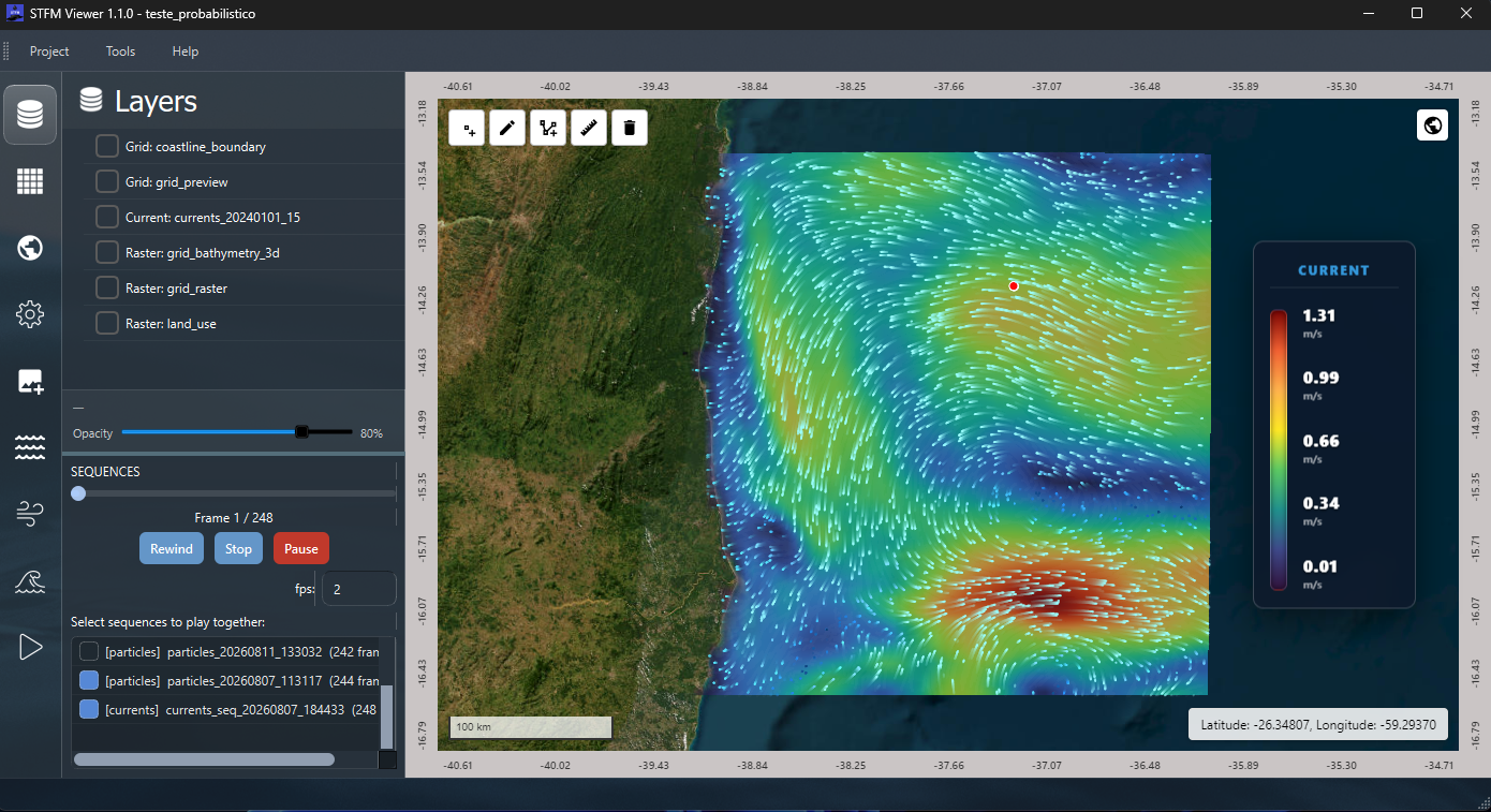
Sequences generated in the Currents, Winds, and Waves panels appear in the panel's Sequences section. Multiple sequences can be active at the same time: for example, viewing animated ocean currents together with the spill point to understand which direction the slick will move.
Figure 7: Current and spill point sequences active at the same time
6. Panel: Grids
The Grids panel creates the computational grid that defines the geographic area and spatial resolution of the simulation. Each grid cell represents a region of the ocean where the model will calculate the position of the oil particles.
The grid must be created before using the Converter and Land Use panels, since both depend on it to clip data to the correct area.
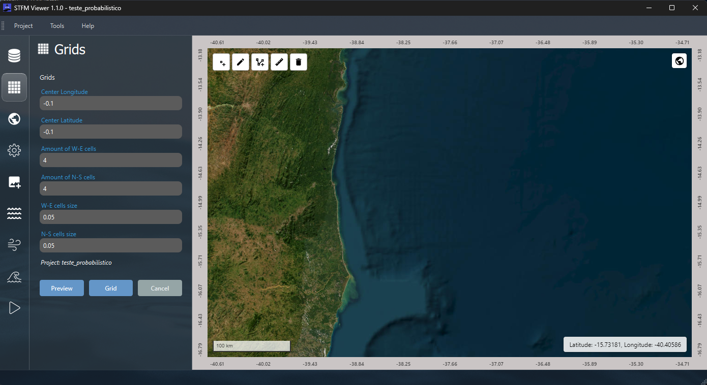
Click the Grids icon in the sidebar to open the panel.
Figure 8: Grids panel
Fill in the grid fields:
Center longitude and latitude: coordinates of the center point of the area of interest, in decimal degrees (e.g., -23.5, -43.2)
Number of W-E cells: number of cells along the east-west axis
Number of N-S cells: number of cells along the north-south axis
Cell size: spatial resolution of each cell, in meters or kilometers: smaller cells increase detail but also processing time
Click Preview to view the grid on the map before generating it. Check that it covers the whole area the slick could reach during the simulation.
If you need to adjust the position or size, click Design. The grid corners become draggable directly on the map. Move them until they fit the correct region.
Once the grid is correct, click Generate. The grid is generated with automatic coastline clipping, and the files are saved to the project's GRIDS/ folder.
Figure 9: Generated grid shown on the map
7. Panel: Land Use
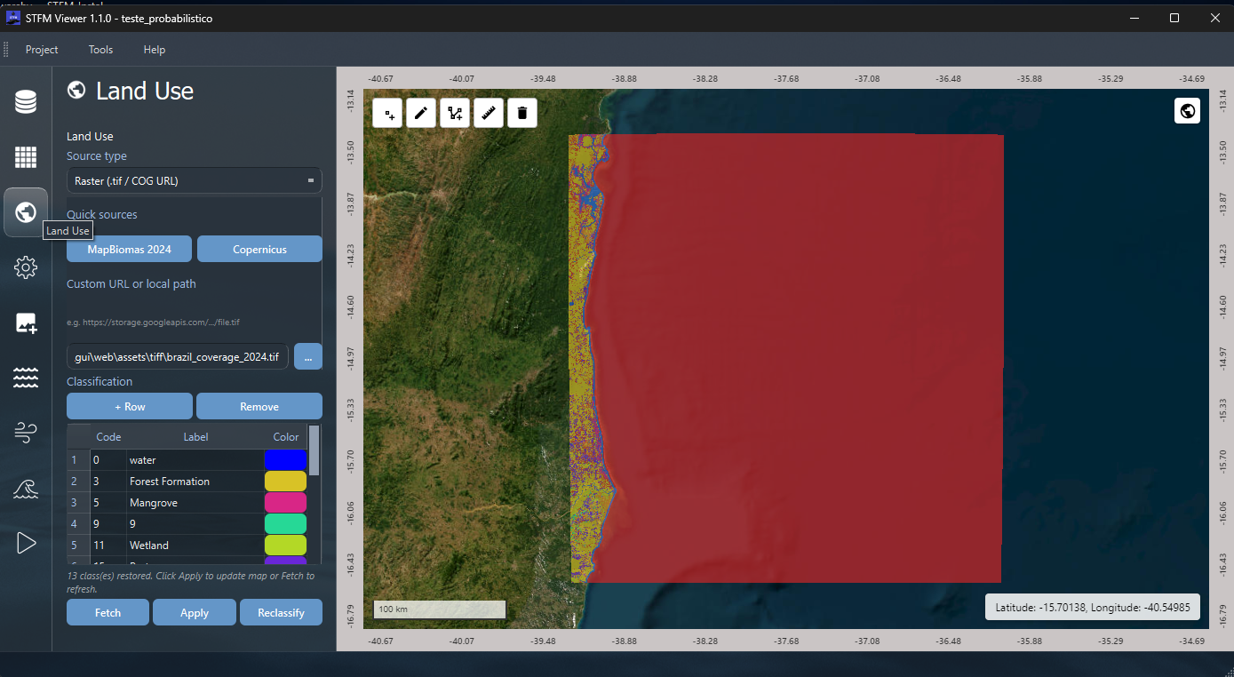
The Land Use panel classifies land cover within the grid area, identifying which cells are water and which are land. This information is used by the simulation to detect when oil particles reach the coast and to calculate the spill's coastal distribution.
Requires that the grid has already been generated in the Grids panel.
Click the Land Use icon in the sidebar to open the panel.
Figure 10: Land Use panel
In the source selector, choose one of the available options:
MapBiomas: land use dataset for South America
Copernicus WCS: global land cover service from the Copernicus programme
ESA WorldCover: high-resolution global mapping from the European Space Agency
Custom URL: paste the address of an external WCS service in the field that appears
Click Fetch. STFM downloads the land cover data for the grid area and displays a classification table with the codes found, their labels, and colors.
Review the table. If you want to adjust a class, edit its label or color directly in the table.
Click Apply to apply the classification and display the result on the map.
To reclassify a specific area:
In some cases the automatic classification may not correctly represent a region: for example, a coastal lagoon classified as land, or a mangrove classified incorrectly. To fix this:
On the map, use the draw polygon button to delimit the area you want to reclassify.
With the polygon drawn, select the new desired classification.
Click Reclassify to apply the new class only to the delimited area. All other cells remain unchanged.
8. Panel: Settings
The Settings panel brings together all the parameters that define the simulation: when and where the spill occurs, how much oil was released, the physicochemical properties of the oil, and which physical processes should be calculated. It is divided into three tabs: Basic Configuration, Oil Properties, and Draw Slick.
Click the Settings icon in the sidebar to open the panel.
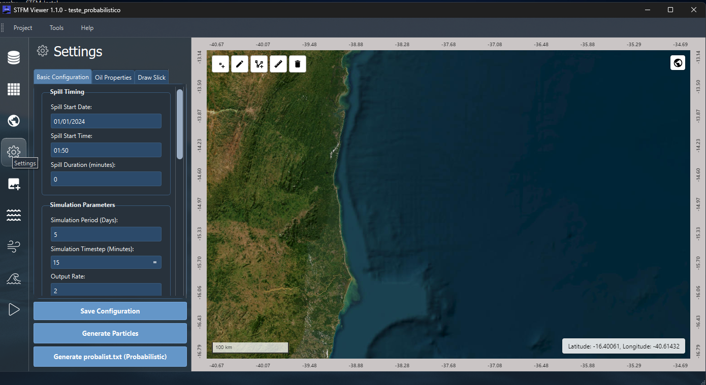
Tab 1: Basic Configuration
Click the Basic Configuration tab.
Figure 11: Settings – Basic Configuration tab
Spill Timing
Defines when the spill occurred or will occur. These values must match the period covered by the downloaded currents, winds, and waves data.
In Spill Start Date, click the field and select the spill's start date.
In Spill Start Time, set the start time in UTC.
In Spill Duration (minutes), enter the total leak duration in minutes. For an instantaneous spill, use 0 or 1. For continuous leaks (a ruptured pipeline, a collapsed well), use the event's actual duration.
Simulation Parameters
In Simulation Period (Days), enter how many days the model should track the slick after the spill. Crude oil slicks can remain visible and active for days to weeks, depending on the oil type and sea conditions.
In Simulation Timestep (Minutes), select the interval between each calculation: 1, 2, 3, 5, 10, 15, 30, or 60 minutes. Smaller intervals increase accuracy, especially in regions with strong or variable currents.
In Output Rate, define how often, in timesteps, results are written. For example, with a 10-minute timestep and an output rate of 6, results are written every hour.
Model Configuration
In Model Dimensions, select:
2D: simulates surface transport only, on the ocean surface : suitable for most surface spills
3D: also simulates transport at depth: required when there is significant droplet dispersion in the water column, and requires current data at multiple depth layers
In Model Type, choose between:
Deterministic: runs a single simulation with the given conditions, producing one defined slick trajectory. Suited to analyzing a specific event with real data.
Time-reverse: runs the simulation backward in time. Suited to identifying the origin of an already-observed slick: it starts from the current position and traces back where the oil came from.
Probabilistic: runs multiple simulations with small variations in initial conditions (different spill start times). The result is a probability map of oil presence in each grid cell: best suited to contingency planning and area risk analysis.
In Runtime Check, leave it Off for normal use. Select Low or High to enable diagnostics during the simulation: useful for identifying numerical instabilities, but increases processing time.
In Interpolation Method, select the method used to interpolate environmental fields between the timestamps of the input data.
Environmental Forcings
Check the forcings that will be included in the simulation. Each forcing uses the converted data from its respective project folder:
Currents: ocean currents: the main driver of the slick's trajectory
Winds: winds: contribute directly to slick transport (about 3% of the surface wind speed) and intensify evaporation and wave-driven dispersion
Temp-Salt: temperature and salinity: used in 3D simulations and for temperature-dependent evaporation calculations
Waves: waves: influence the dispersion of oil droplets into the water column (entrainment) and add extra drift speed (Stokes drift)
Mandatory forcing rules:
Currents and Winds are always required. It is not possible to generate the timestamp file or run the simulation without both. Any other combination (Currents only, Winds only, Waves only, etc.) will be rejected.
Waves and Temp-Salt are optional, and can be used in any combination alongside Currents and Winds.
All checked forcings must share the same timestamps. The files converted into the CURRENTS/, WINDS/, WAVES/, and TEMPERATURE/ folders need to cover exactly the same times. If the current files cover a different period than the wind files, generating the timestamp file will fail with a message indicating which times are missing from each folder.
In Longitude and Latitude, enter the spill point coordinates in negative decimal degrees for South/West (e.g., -23.50 and -43.20).
In Depth (m), enter the spill depth. For surface spills (tanker, coastal pipeline), use 0. For subsea well spills, enter the water depth.
In Volume (Metric Ton), enter the total volume of oil spilled, in metric tons.
In Number of Lagrangian Particles, set how many particles will represent the slick. Each particle represents a fraction of the total oil volume. More particles produce more detailed, smoother results, but increase processing time. Values between 1,000 and 10,000 are common.
Tab 2: Oil Properties
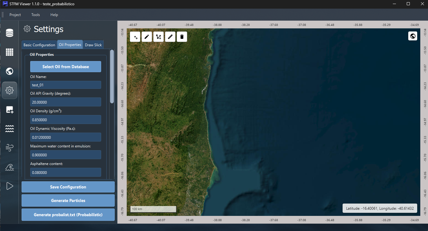
The physicochemical properties of the oil determine how it behaves after the spill: how fast it evaporates, whether it forms a stable emulsion with seawater, how viscous it becomes over time, and how long it stays on the surface. Light oils (high API) evaporate quickly and leave little residue. Heavy oils (low API) evaporate little, form dense and viscous emulsions, and persist on the surface for much longer.
Click the Oil Properties tab.
Figure 12: Settings – Oil Properties tab
To select an oil from the database:
Click Select Oil from Database.
In the window that opens, search for the desired oil type by name (e.g., Arabian Light, Marlim, Petrobras) and click it to select it.
The fields below are filled in automatically with the measured values for that oil:
API Gravity: a scale that measures oil density: values above 31° indicate light oils, below 22° indicate heavy oils
Density: oil density in kg/m³
Viscosity: the oil's resistance to flow: highly viscous oils spread more slowly and are harder to remove
Asphaltene content: asphaltene content: heavy compounds that stabilize water-in-oil emulsions; oils with a high asphaltene content tend to form thick, persistent emulsions
Water content: initial water content present in the oil
Evaporation and emulsification constants characteristic of that oil type
To fill in manually:
If the oil type is not in the database, enter the values directly in each field. Refer to the oil's technical data sheets or lab analysis reports.
Numerical coefficients:
Horizontal Diffusion Coefficient: represents the horizontal turbulent dispersion of the particles: controls how much the slick spreads over time due to ocean turbulence
Windage Coefficient: the fraction of wind speed transferred directly to the slick's movement: typically between 2% and 4%
Current Drag Coefficient: the fraction of surface current speed used in slick transport: typically 100%
Weathering processes:
Check the physical processes that should be calculated during the simulation. Each process consumes fractions of the spilled oil or changes its properties over time:
Spreading: the slick expands horizontally: gravity tends to spread it while viscosity resists; directly affects the covered area and slick thickness
Evaporation: the lighter fractions of the oil vaporize into the atmosphere: this is the most significant weathering process by volume; light oils can lose 50–60% of their mass within a few hours, while heavy oils lose less than 10% over days
Emulsification: droplets of seawater penetrate the oil, forming a stable mixture that can reach 80% water: significantly increases the slick's apparent volume and makes the oil denser and more viscous; oils with more asphaltenes form more stable and persistent emulsions
Dissolution: soluble fractions of the oil dissolve into the water column: represents a small mass loss (less than 1%), but the dissolved compounds (aromatic hydrocarbons) are toxic to marine life even at low concentrations
Entrainment: oil droplets are mechanically dispersed into the water column by breaking waves: oil that does not return to the surface is removed from the slick and transported below it
Tab 3: Draw Slick
The Draw Slick tab lets you place the oil particles on the map before starting the simulation. The spill can be represented as a single point or as a distributed area, depending on how the accident occurred.
Click the Draw Slick tab.
Figure 13: Settings – Draw Slick tab
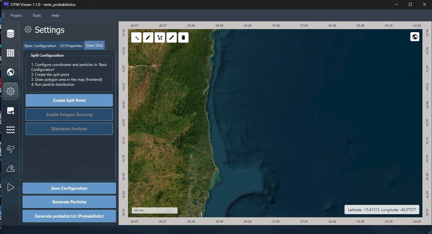
Step 1: Create the spill point
Click Create Spill Point.
If the coordinates are already filled in on Tab 1, the point is created automatically on the map at the correct position.
If they are not filled in, the cursor switches to selection mode: click on the map at the exact spill location.
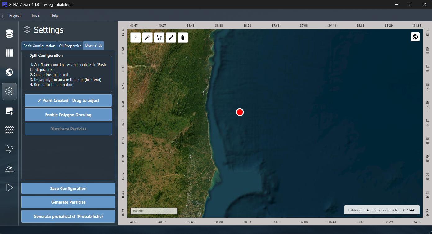
The point appears on the map. If you need to adjust its position, drag it directly on the map: the coordinates on Tab 1 are updated automatically.
Figure 14: Spill point created on the map
Step 2: Draw the spill area
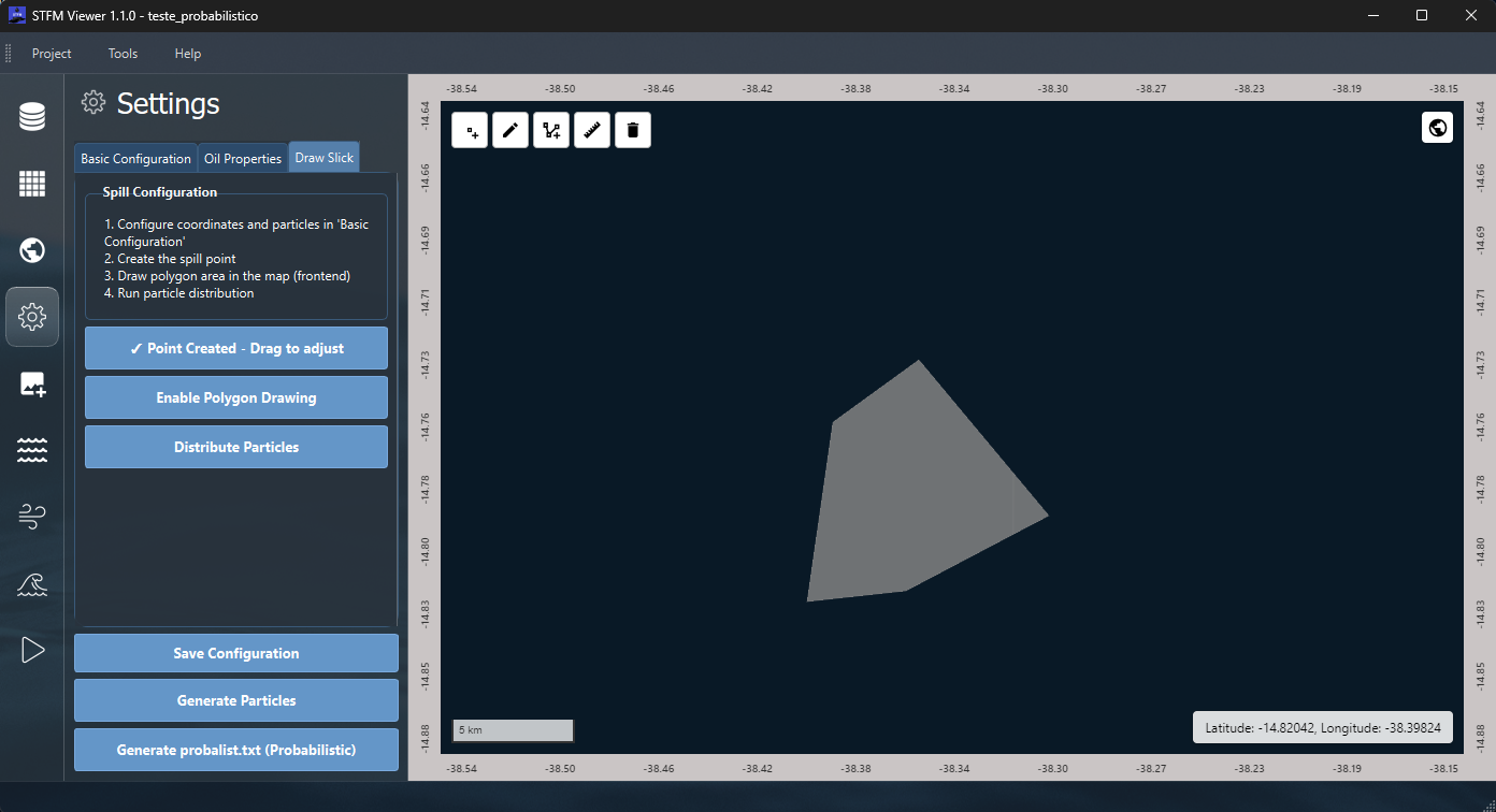
When the spill has already occurred and the slick has a known extent (from satellite imagery or an overflight, for example), you can delimit that area so particles are distributed within it, representing the slick's real condition at the start of the simulation.
Click Enable Polygon Drawing (available only after the point has been created).
On the map, click the vertices of the observed slick's area. When finished, close the polygon by clicking on the starting point.
The polygon appears highlighted on the map, delimiting the spill area.
Figure 15: Spill polygon drawn on the map
Step 3: Distribute the particles
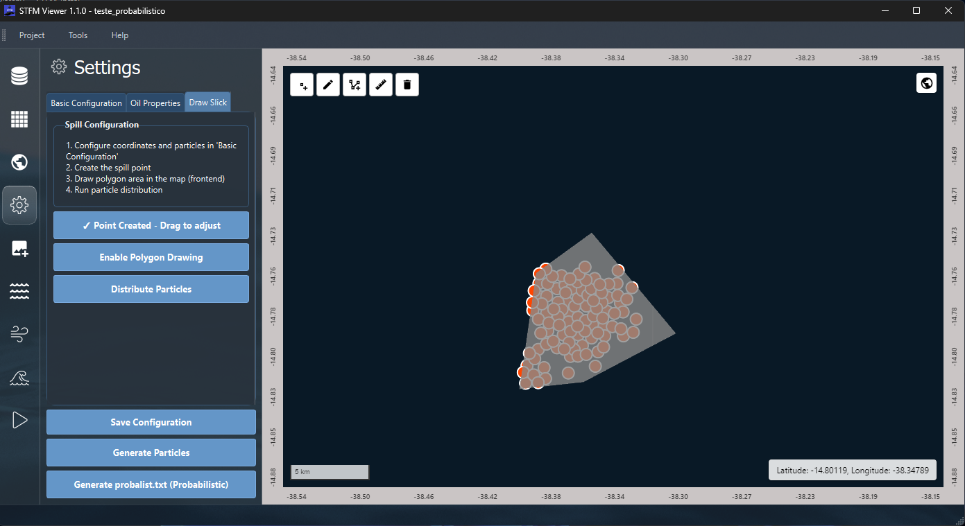
Click Distribute Particles (available only after the polygon has been drawn).
The particles are distributed within the polygon and shown on the map. The number of particles is the same as defined on Tab 1, under Number of Lagrangian Particles.
Figure 16: Particles distributed on the map
Saving and generating
After configuring the three tabs:
Click Save Configuration to save all parameters to the project's CONFIG/ folder.
Click Generate Particles if you prefer to generate particles concentrated at the coordinate point from Tab 1, without using the polygon: suitable for point-source spills (e.g., a well or a ship).
If the model is in Probabilistic mode, click Generate probalist.txt to generate the file with the draw instants used across the multiple simulations.
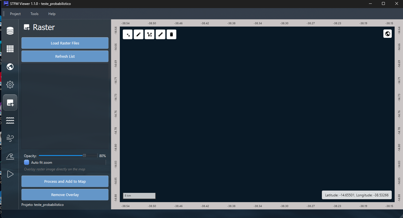
9. Panel: Raster
The Raster panel lets you overlay georeferenced images on the map for comparison or visual reference: for example, a satellite image of the observed slick or a bathymetric map of the region.
Click the Raster icon in the sidebar to open the panel.
Figure 17: Raster panel
Click Load Raster Files and select the desired image (GeoTIFF or similar formats).
Click Refresh List if you need to update the file list.
Adjust the opacity with the slider to overlay the image on the base map.
If you want the map to automatically zoom to the image's extent, check Auto fit zoom.
Click Process and Add to Map to display the image on the map.
To remove the image from the map, click Remove Overlay.
10. Tools: Downloader
The Downloader downloads the oceanographic and meteorological data used as forcings for the simulation: ocean currents (HYCOM), atmospheric winds (GFS), and waves (Copernicus Marine). Data is downloaded for the period of interest and saved to the project's RAW_DATA/ folder.
In the top bar, click Tools.
Click Downloader. The Downloader opens in a separate window.
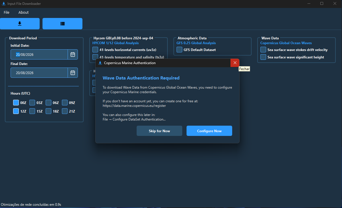
Figure 18: Downloader main screen
Available data sources
Source
Data
Use in the simulation
HYCOM
Ocean currents at multiple depths, temperature and salinity
Main driver of the slick's trajectory
GFS
Surface atmospheric winds
Additional slick drift (~3% of wind speed) and evaporation
Copernicus Marine
Significant wave height and Stokes drift
Dispersion of oil droplets and wave-driven drift
Step by step
1. Select the destination folder
On the first screen, click Browse, navigate to the project's RAW_DATA/ folder, and confirm.
2. Configure Copernicus credentials
If you will be downloading wave data, an authentication window appears automatically. Enter your Copernicus Marine username and password and click Configure Now. If you don't have an account, visit marine.copernicus.eu to create one. If you'd rather configure it later, click Skip for Now.
3. Set the period
Click the Initial Date field and select the start date: it must be equal to or earlier than the spill date configured in Settings.
Click the Final Date field and select the end date: it must cover the entire simulation period configured in Settings.
4. Select the times
Check the UTC times you want to download: 00Z, 03Z, 06Z, 09Z, 12Z, 15Z, 18Z, 21Z. The more times you include, the better the representation of current and wind variability throughout the day, especially in regions with tides or coastal breezes.
5. Select the variables
For each source, check the desired variables:
HYCOM: check 41-levels horizontal currents (uv3z) for currents and/or 41-levels temperature and salinity (ts3z) for temperature and salinity (needed for 3D simulations and for temperature-dependent evaporation)
GFS: check GFS Default Dataset for atmospheric wind data
Copernicus: check Sea surface wave stokes drift velocity for the wave-driven Stokes drift and/or Sea surface wave significant height for wave height (used to calculate droplet dispersion)
6. Start the download
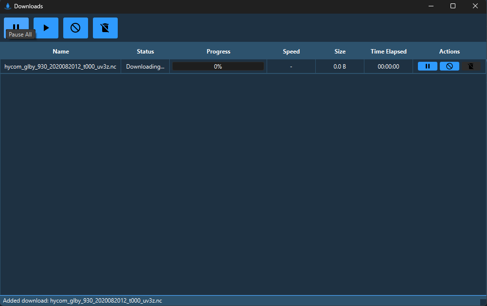
Click the download button (down-arrow icon at the top of the screen). The progress window opens.
Figure 19: Downloader progress screen
Track progress in the table. For each file you can:
Click the pause button to pause the download
Click the cancel button to stop it
Wait until the status changes to Completed
7. Interrupted downloads
If a download is interrupted, its state is saved automatically. The next time you open the Downloader, it will ask if you want to resume. Downloads older than 7 days are not resumed.
11. Tools: Converter
The Converter adapts the raw data downloaded by the Downloader to the format, area, and resolution of the project's grid. The original data covers large portions of the ocean and needs to be clipped and reformatted to fit the grid defined in the Grids panel.
In the top bar, click Tools.
Click Converter. The Converter opens in a separate window.
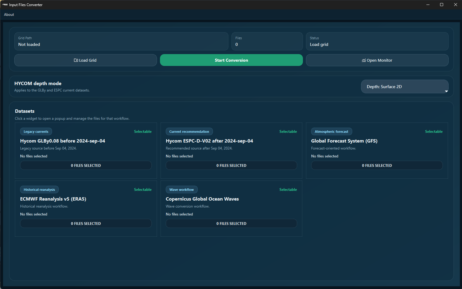
Figure 20: Converter screen
Step by step
1. Load the grid
Click Load Grid.
Browse to the project's GRIDS/ folder, select the grid file, and click Open.
The Grid Path field is filled in and the status confirms the grid was loaded. From this point on, the Converter knows which area to clip the data to.
2. Select the data to convert
The Converter displays cards for each available data type. Click the card corresponding to the files you want to convert:
Hycom GLBy0.08 before 2024-sep-04: for HYCOM currents downloaded before September 2024
Hycom ESPC-D-V02 after 2024-sep-04: for HYCOM currents downloaded after September 2024 (new version of the HYCOM model)
Global Forecast System (GFS): for GFS wind data
ECMWF Reanalysis v5 (ERA5): for ECMWF reanalysis (high-quality historical data)
Copernicus Global Ocean Waves: for Copernicus Marine wave data
Clicking a card opens a window to select the files downloaded into the RAW_DATA/ folder. Select the files and confirm.
3. Select the depth (HYCOM only)
In the HYCOM depth mode selector, choose:
Surface 2D: extracts surface-only ocean data: use when the model is configured for 2D in Settings
Multi-level 3D: extracts data across multiple depth layers: use when the model is configured for 3D, to simulate the transport of oil dispersed below the surface
4. Start the conversion
Click Start Conversion.
To monitor progress, click Open Monitor.
When finished, the converted files are automatically saved to the project's CURRENTS/, WINDS/, or WAVES/ folders, ready to be loaded into the corresponding panels.
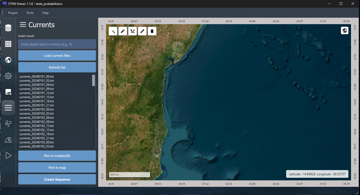
12. Panel: Currents
The Currents panel loads the converted ocean current data and lets you view it on the map before the simulation. Currents are the main driver of the oil slick's trajectory.
Click the Currents icon in the sidebar to open the panel.
Figure 21: Currents panel
In the Input level field, enter the depth level in meters you want to view (use 0 for the surface).
Click Load current files. Files from the project's CURRENTS/ folder are loaded into the list.
If the files don't appear, click Refresh All.
Select the desired file from the list.
Click Plot to map to display the current field on the interactive map: vectors show direction and magnitude.
To generate an animation showing how currents evolve over time, select all the desired files and click Create Sequence. The sequence will be available in the Layers panel for playback.
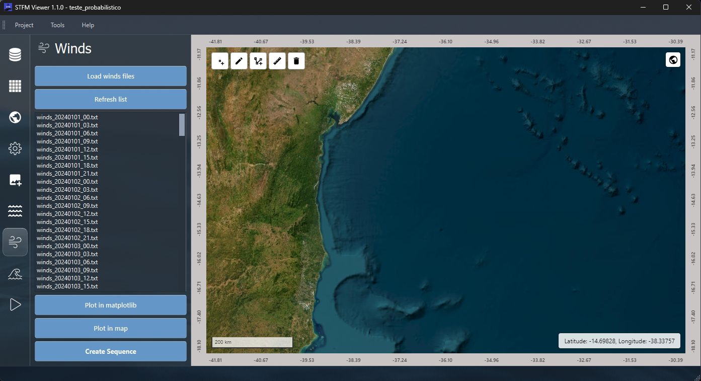
13. Panel: Winds
The Winds panel loads the converted wind data and lets you view it on the map. Winds contribute directly to the slick's drift (about 3% of the surface wind speed) and intensify evaporation of the oil's lighter fractions.
Click the Winds icon in the sidebar to open the panel.
Figure 22: Winds panel
Click Load wind files. Files from the project's WINDS/ folder are loaded into the list.
If the files don't appear, click Refresh All.
Select the desired file from the list.
Click Plot to map to display the wind field on the interactive map.
To generate an animation, select all the desired files and click Create Sequence. The sequence will be available in the Layers panel for playback.
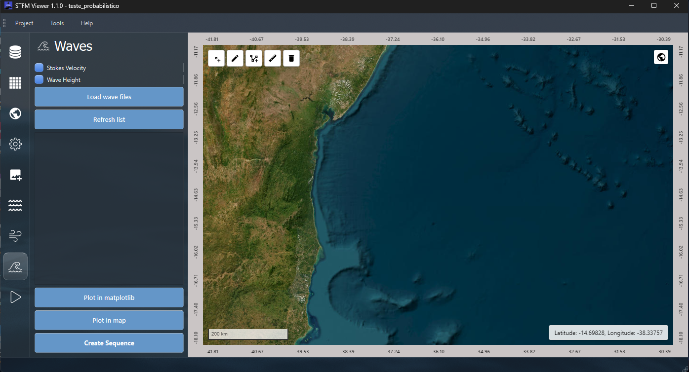
14. Panel: Waves
The Waves panel loads the converted wave data and lets you view it. Waves act on the simulation in two ways: Stokes drift (extra drift generated by waves) moves the slick, and wave height determines the intensity of oil droplet dispersion in the water column: larger waves disperse more oil below the surface, reducing the visible slick area more quickly.
Click the Waves icon in the sidebar to open the panel.
Figure 23: Waves panel
Check the variables you want to view:
Stokes Waves: Stokes drift: the drift velocity of water particles generated by waves, in their direction of propagation
Wave Height: significant wave height: the average of the highest third of the waves measured at that location
Click Load wave files. Files from the project's WAVES/ folder are loaded into the list.
If the files don't appear, click Refresh All.
Select the desired file from the list.
Click Plot in oceanography to open the static view of the wave variables.
Click Plot to map to display the waves on the interactive map.
To generate an animation, select all the desired files and click Create Sequence. The sequence will be available in the Layers panel for playback.
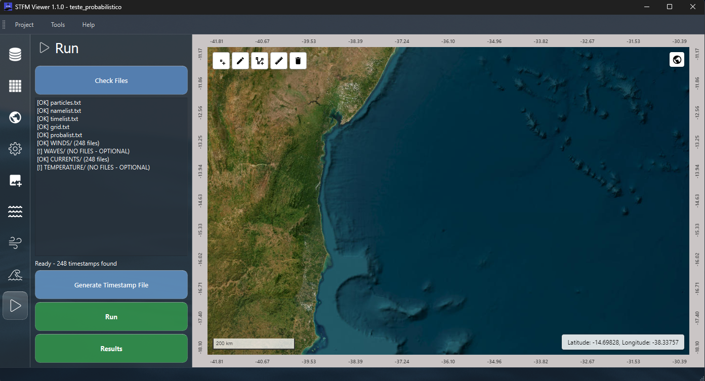
15. Panel: Run
The Run panel checks that all required files are present and runs the simulation.
Click the Run icon in the sidebar to open the panel.
A checklist is displayed automatically with the items required for the simulation. Items marked OPTIONAL are not required to run it.
Figure 24: Run panel with checklist
1. Check the files
Click Check Files to refresh the checklist.
Verify that all required items are marked as present.
If a required item is missing, go back to the corresponding panel to generate it before proceeding:
Grid missing: go back to the Grids panel
Configuration missing: go back to Settings and save
Currents missing: go back to Currents and load the files
Winds or waves missing (if checked as forcings in Settings): go back to the Winds or Waves panels
2. Generate the timestamp file
Click Generate Timestamp File to generate the file with the simulation's time instants, calculated from the parameters configured in Settings (start date, period, and timestep).
3. Run the simulation
Click Run to start the solver.
Wait for it to finish. Progress is shown on screen. Long simulations (several days, probabilistic mode with many realizations) can take a few minutes.
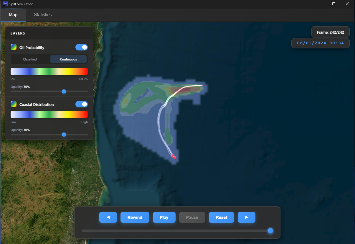
4. View the results
When it finishes, click Results to open the results viewer.
Figure 25: Results viewer
In the viewer:
Use the playback controls at the bottom to play, pause, or step forward/backward frame by frame through the simulation timeline.
In the left panel, toggle the available layers:
Oil Probability: a map of the probability of oil presence in each grid cell: generated in Probabilistic mode; each cell shows the fraction of realizations in which oil passed through it, indicating higher-risk contamination areas
Coastal Distribution: distribution of oil along coastal segments: shows which stretches of coastline were reached by particles and in what quantity, allowing response and cleanup actions to be prioritized
The counter in the upper-right corner shows the current frame and the corresponding date/time in the simulation.
More Guides
Environmental data, in depth
Dedicated deep dives on the Downloader and Converter, plus manual alternatives for when they're not an option.
STFM Tools
Downloader Guide
Fetch HYCOM, GFS, and Copernicus Marine data automatically.