About the Model

How STFM sees a spill

STFM represents a spill as thousands of individual particles, each carrying its own position, volume, and oil properties moved and transformed step by step as physical processes act on them.

A particle-based view

Instead of tracking a spill as a single blob, STFM splits it into a large number of Lagrangian particles typically thousands per simulation. Each particle carries its own mass, volume, thickness, and oil properties, and is moved individually at every timestep in response to the currents, winds, and waves at its exact position.

This is what lets one model cover both scales at once: near the source, particles behave according to near-field physics; as they spread out, the same particles respond to far-field forcing with no hand-off between separate tools.
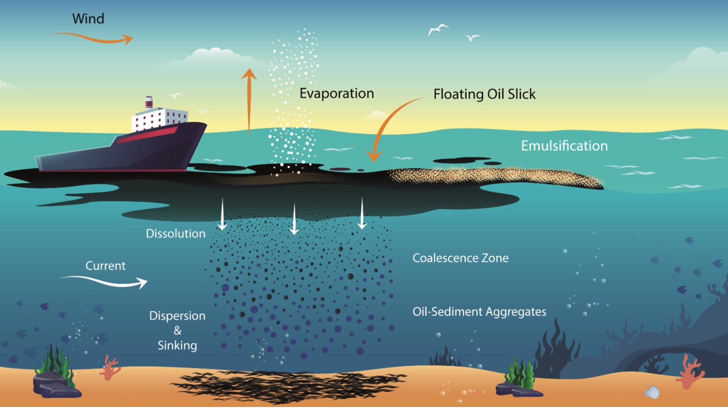
Diagram of oil weathering processes: evaporation, emulsification, dissolution, and dispersion into the water column
How a slick evolves after release: evaporation at the surface, emulsification with seawater, dissolution, and dispersion into the water column.

Two scales, one model

Most transport models are tuned for one regime. STFM moves between both:

  • Near-field — captures the turbulence and buoyancy that dominate close to a release, where jet and plume behavior set the starting condition for everything downstream.
  • Far-field — tracks advection and dispersion outward across hours to days, driven by ambient currents, wind, and tidal forcing rather than the source itself.

A model can be run in 2D (surface transport only, suitable for most surface spills) or 3D (also tracking movement at depth, using current data across multiple depth layers) set once, before the run, depending on how much the spill is expected to disperse below the surface.

What moves the oil

Each particle's position updates every timestep from three combined effects:

  • Advection — the particle is carried by a weighted combination of surface current, wind, and wave-driven (Stokes) drift, following a scheme adapted from established tidal and surface-drift modeling literature.
  • Turbulent diffusion — a random-walk component adds the small-scale spreading caused by ocean turbulence, so identical particles released together don't all take the exact same path.
  • Mechanical spreading — the slick spreads horizontally over time as gravity pulls it outward and viscosity resists, following a formulation from published Adriatic Sea spill modeling work.

Together, these three effects are what separate a wind-driven spill from a current-driven one, and what determine how tight or diffuse a slick looks after a few hours versus a few days.

Real tooling, not just theory

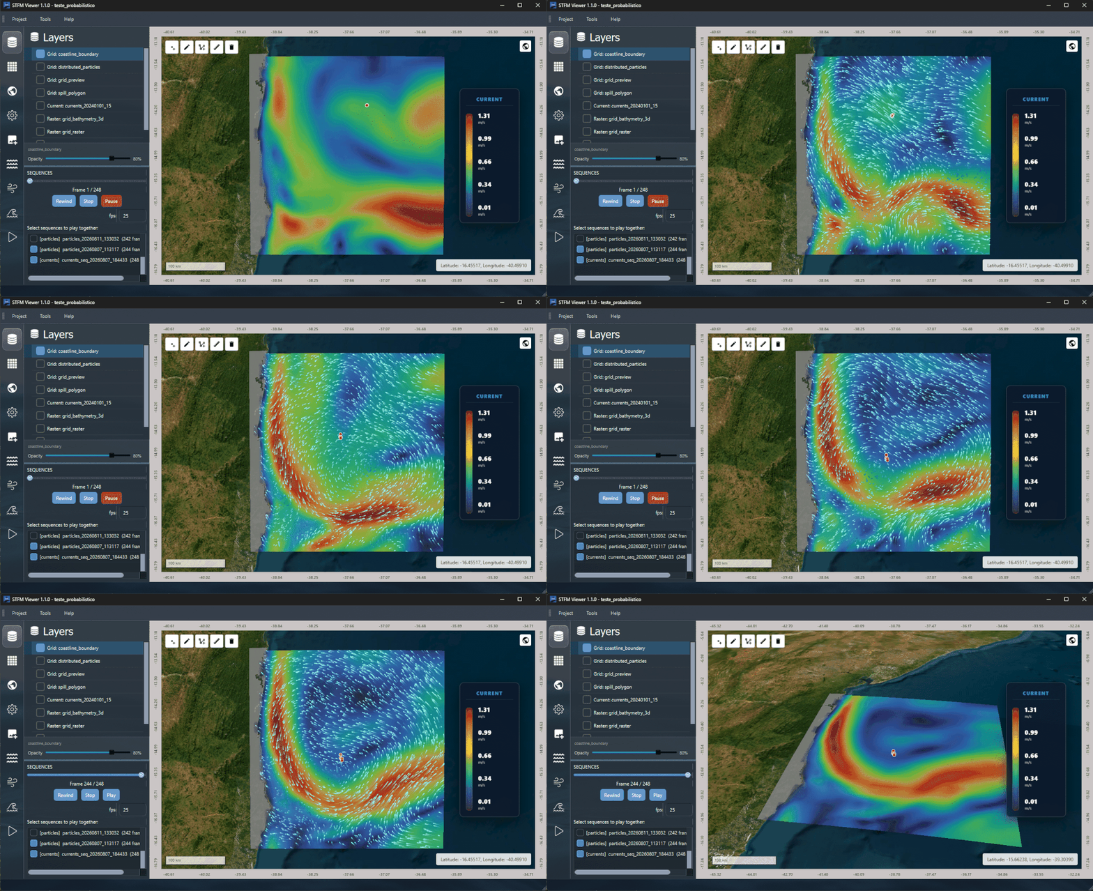
Every process described above is something you can actually see move, inside the STFM Viewer not a static output file to interpret after the fact.

Animated sequence of ocean current fields playing back over time in the STFM Viewer's Layers panel

Currents over time

Multiple current snapshots stitched into a sequence, playable directly on the grid.
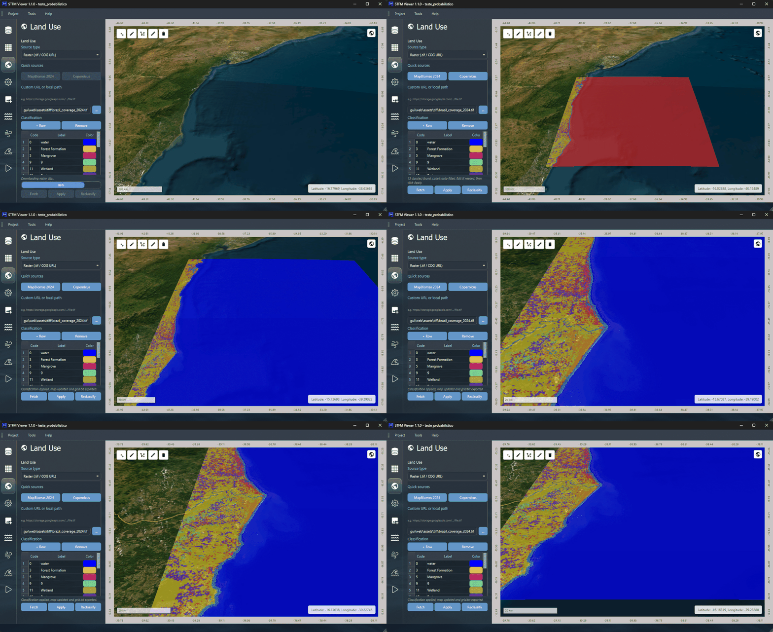
Land use classification workflow in the STFM Viewer, showing source selection and a coded classification table

Coastline, classified

Land use sources like MapBiomas or Copernicus define exactly where "coast" begins for the model.

How the oil changes over time

Alongside transport, STFM tracks how the oil itself changes each particle's mass and volume shrink or shift as these processes act on it, each based on a specific published formulation:

  • Evaporation — the lighter fractions vaporize into the atmosphere, following a parametrization from the reference textbook Oil Spill Science and Technology (Fingas). This is usually the largest single mass loss in the first hours after a spill.
  • Dissolution — soluble compounds dissolve into the water column, based on a published model for predicting dissolution rates of toxic compounds from spilled oil. A small fraction of the total mass, but ecologically significant even at low concentrations.
  • Emulsification — seawater droplets work into the oil, following a formulation from recent published research on modeling emulsification's influence on oil properties and spill response. This raises viscosity and can markedly increase the oil's apparent volume.
  • Dispersion — wind-driven wave action breaks part of the slick into droplets that mix into the water column, calculated from the oil's viscosity, film thickness, and interfacial tension.

Every process is tied to real-time sea and air temperature, so the same oil weathers differently in a tropical simulation than in a colder one matching what actually happens at sea.

Scenario types

Because release conditions vary so much a surface leak, a subsea rupture, a moving vessel STFM is exercised against a range of spill hypotheses during development and validation. A few examples:
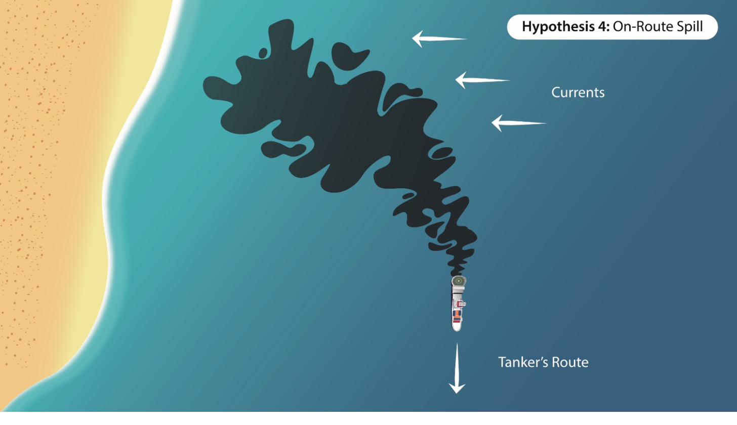
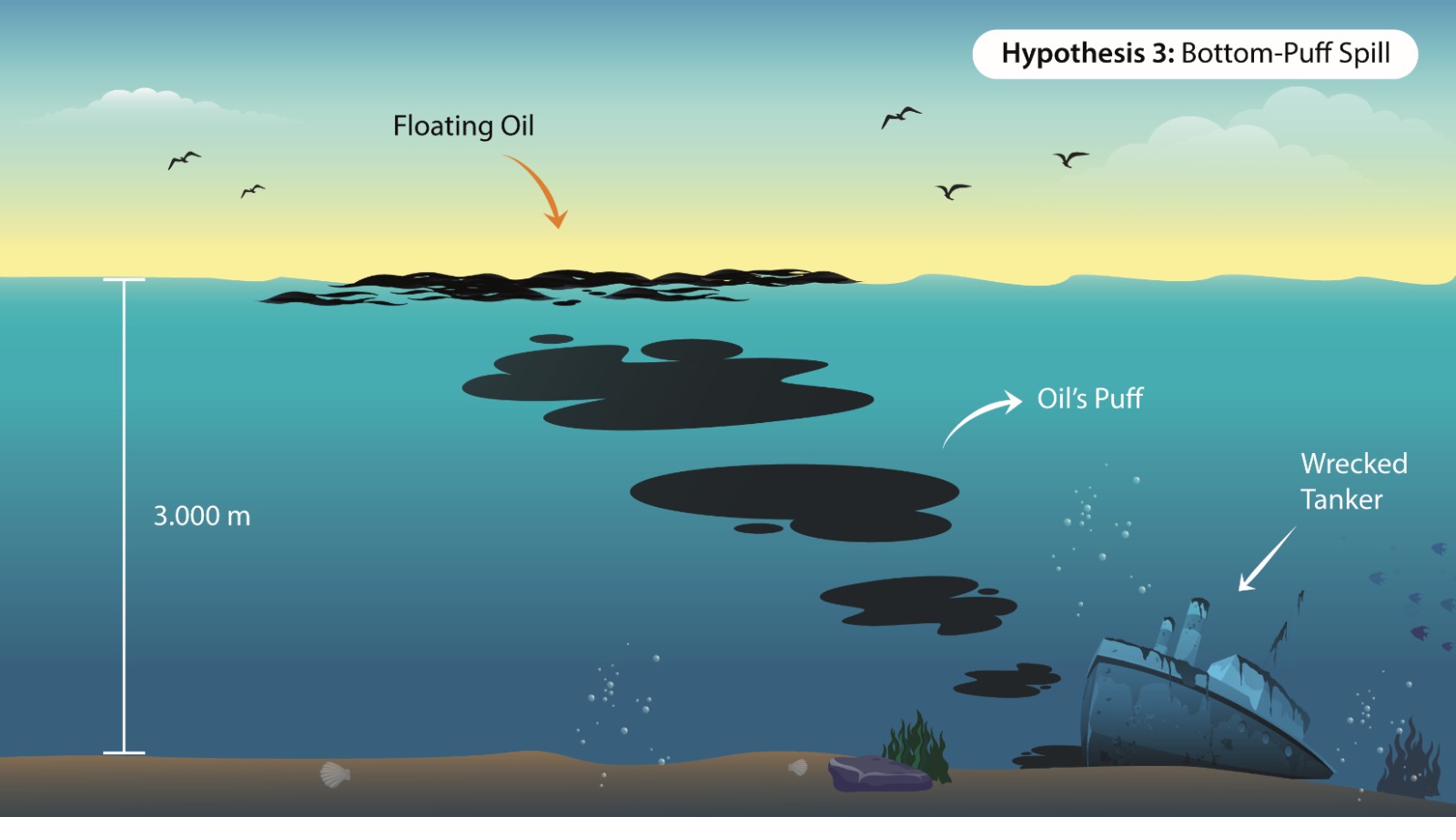
Diagram of an on-route spill from a moving tanker, with the slick trailing behind and spreading under the influence of currents
On-route spill: oil released continuously from a moving vessel, trailing and spreading under ambient currents.
Diagram of a subsea well or wrecked tanker releasing oil in puffs that rise through the water column before reaching the surface
Bottom-release spill: oil rising in puffs from a deep source, dispersing through the water column before reaching the surface.
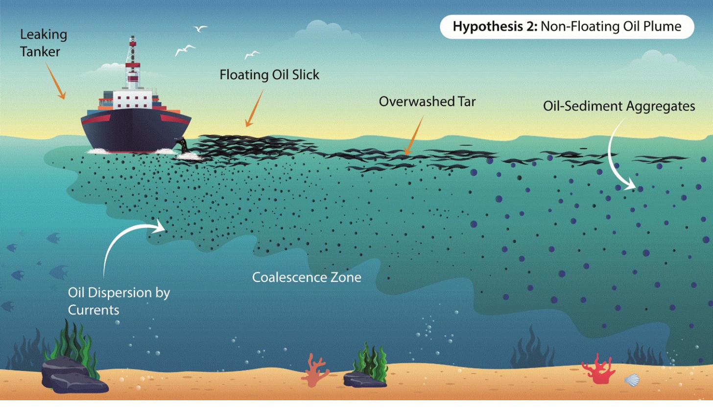
Diagram showing a subsurface, non-floating oil plume dispersed as droplets and oil-sediment aggregates rather than a surface slick
Non-floating plume: oil that disperses as droplets and oil-sediment aggregates in the water column, rather than forming a continuous surface slick.

Three ways to run a simulation

Deterministic

One event, one answer

Runs once with a defined set of conditions, producing a single trajectory. Suited to reconstructing or forecasting one specific event.

Time-reverse

Work backward from what's observed

Runs the physics in reverse from an already-observed slick, tracing back toward a likely source — useful for forensic-style investigation.

Probabilistic

Many runs, one risk map

Runs many times with varied conditions, producing a probability map of oil presence — built for contingency planning and licensing.

Get Started

See it running on real data

Follow the guide to set up SisMOM, or jump straight to the download.